

A fusion design with a lower projected mature electricity cost can still have a less viable commercial path. Its first plants may be too expensive, or its learning rate too slow, to attract enough orders to reach that cost.
Fusion cost claims usually describe the levelized cost of electricity, or LCOE, from two plants: a first-of-a-kind plant, FOAK, and a mature nth-of-a-kind plant, NOAK. An expected learning curve connects them. The learning rate is the percentage cost reduction per doubling of cumulative production. Reaching NOAK requires enough plants to be financed, built and operated for those reductions to occur. Construction time, financing, availability and net output can also change LCOE.
Figure 1 illustrates the problem. Design A starts at $110/MWh and reaches a $65/MWh NOAK. Designs B and C start at $220/MWh and promise a lower $35/MWh NOAK. Yet B stops after 16 plants and C after four because the next customers will not pay enough. A keeps selling. The dashed portions of B and C’s curves require production that the assumed market does not support.
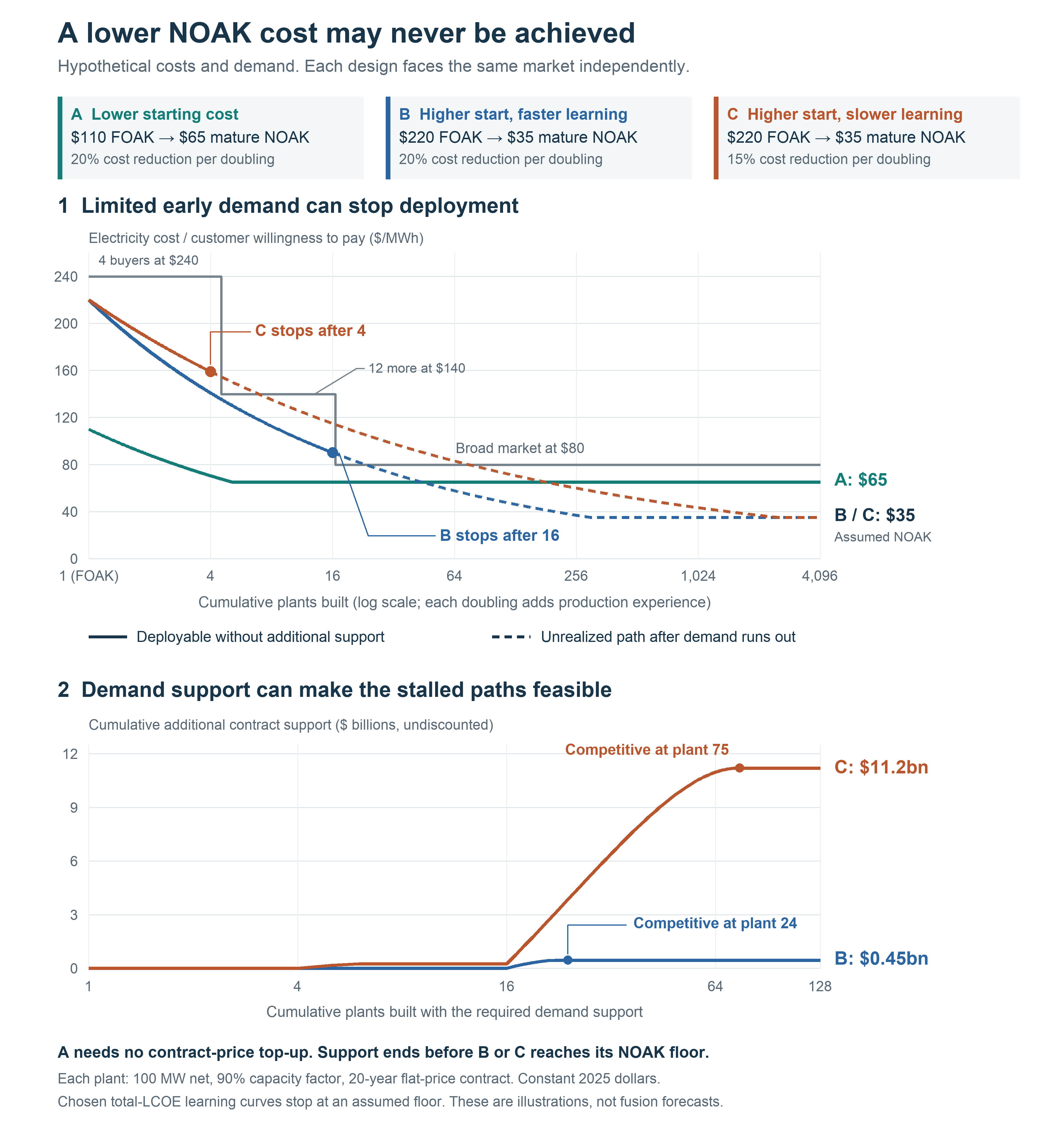
Figure 1. A lower NOAK cost may never be achieved. Solid lines show deployment supported by a hypothetical market; dashed lines require additional support. B and C need about $447 million and $11.2 billion in undiscounted support commitments to reach competitiveness, before reaching NOAK. Each design faces the same demand independently. The calculation assumes 100 MW net plants, 90% capacity factor and 20-year contracts, in constant 2025 dollars. Details appear in the demand-support section and linked model.
If FOAK electricity costs less than comparable substitutes, ordinary demand may support further plants, provided customers and lenders trust them to deliver. If it costs more, enough customers must value other features, or subsidies must cover the gap, until the product becomes competitive. Someone must buy the early output.
For 1cFE, a plausible 1¢/kWh NOAK, or $10/MWh in 2025 dollars, therefore needs an economically plausible path from the first plants. Material multipliers help identify manufacturing costs to investigate. Learning curves connect potential reductions to the production required. Neither establishes that the market will support that production.
What the material multiplier tells us
A high material multiplier identifies costs to investigate. It does not tell us which can be removed. The ratio compares finished-component cost with the commodity value of its constituent materials:
M = C_finished / V_materials
C_finished and V_materials use the same price basis. M is dimensionless. Elon Musk’s name for the ratio, the “idiot index,” was popularized by Walter Isaacson’s biography. Material multiplier is a more useful term because a high ratio can reflect necessary work (Isaacson, 2023).
A pill can be worth far more than its ingredients because of the treatment it provides. Small-molecule brand-name drugs can cost pennies per additional pill to manufacture, while discovery, testing and approval require substantial expenditure. Prices also reflect patents and market power. The multiplier alone measures neither waste nor value (CBO, 2022).
Figure 2 uses two familiar US products:
A passenger car: DOE estimates selling price at about $8 per pound and raw materials at $0.60 per pound, giving about 13. Selling price includes manufacturing, shipping and commercial margins (DOE, 2012).
A single-family house: purchased materials and components account for roughly half of hard construction cost, giving about 2. Land and other development costs are excluded. The denominator already includes upstream manufacturing, so this is not a raw-material multiplier (Potter, 2026).
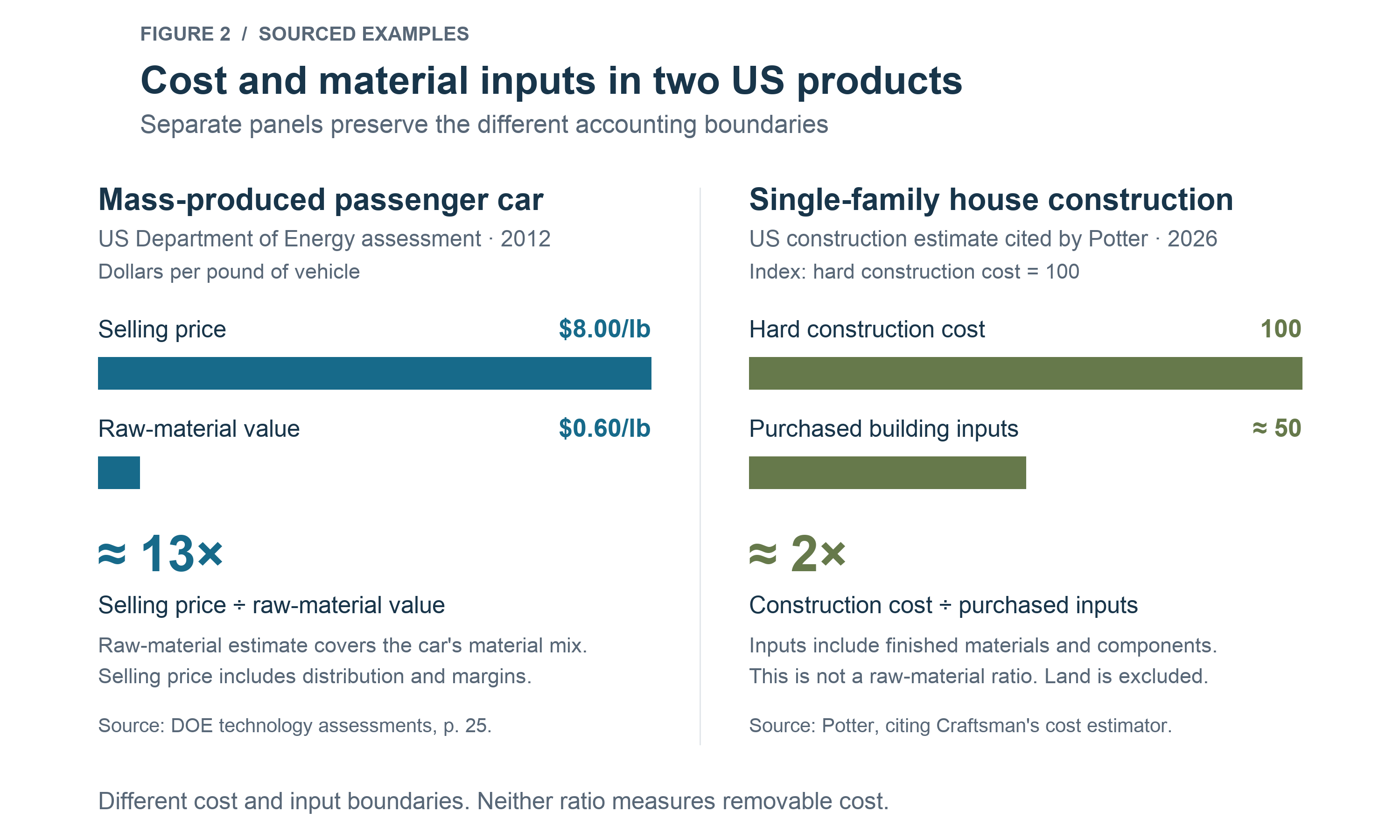
Figure 2. Separate panels retain the car’s raw-material denominator and the house’s purchased-input denominator. These ratios do not rank manufacturing efficiency or measure removable cost. Source locations, arithmetic and limitations are in the accompanying data.
Even mass production leaves substantial cost above a car’s raw-material value. Fabrication, engineering, tooling, inspection, overhead and margins all contribute. Different interventions address different costs: more output spreads development expense, process redesign can reduce scrap, and competition can reduce margins (Potter, 2025). There is no reason to assign the entire difference one improvement mechanism.
For a fixed design and material-price basis, the material bill sets a lower bound on cost. The multiplier sets a ceiling on the possible fractional reduction: cost cannot fall by more than 1 - 1/M without going below that bill. Necessary processing and qualification make the attainable saving smaller. A breakthrough in raw-material production can lower the bill itself, as can a design that uses less material or substitutes a cheaper one.
The multiplier says nothing about whether repeated projects will shorten permitting or regulatory review. Those improvements can reduce delays and financing costs without changing the material bill.
Fusion magnets require particular care. Their material inventory includes substrate, stabilizer and structure, not just rare-earth compounds. Purchased rare-earth barium copper oxide (REBCO) superconducting tape already contains manufacturing work. Completed-magnet cost divided by purchased-tape cost measures assembly and procurement additions, not the raw-material multiplier. These boundaries distinguish a reduction in tape quantity from a cheaper tape-manufacturing or magnet-assembly process.
Learning needs a floor and a production count
A large material multiplier can coexist with a demanding production requirement. Consider a magnet costing $10 million, with a $200,000 constituent-material bill and an assumed $1 million engineering floor. Its material multiplier is 50. If the cost above that floor falls by 20% per production doubling, reaching $2 million still requires about 9.85 doublings, or about 920 times the reference cumulative production.
The engineering floor, F, includes the materials and necessary processing remaining under a stated design, performance requirement and input-price basis. It is distinct from the raw-material bill. A different design or production process can change it. A constant percentage reduction in total cost eventually predicts costs below these requirements, so we separate the cost above F and call it the residual.
After D doublings, with reference cost C_0 and residual learning rate r_res:
C(D) = F + (C_0-F) × (1-r_res)^D
In the magnet example, the residual starts at $9 million. Cost reaches about $5.61 million after three doublings and $3.36 million after six. Each doubling removes 20% of the remaining residual, so the percentage reduction in total cost gets smaller as it approaches F.
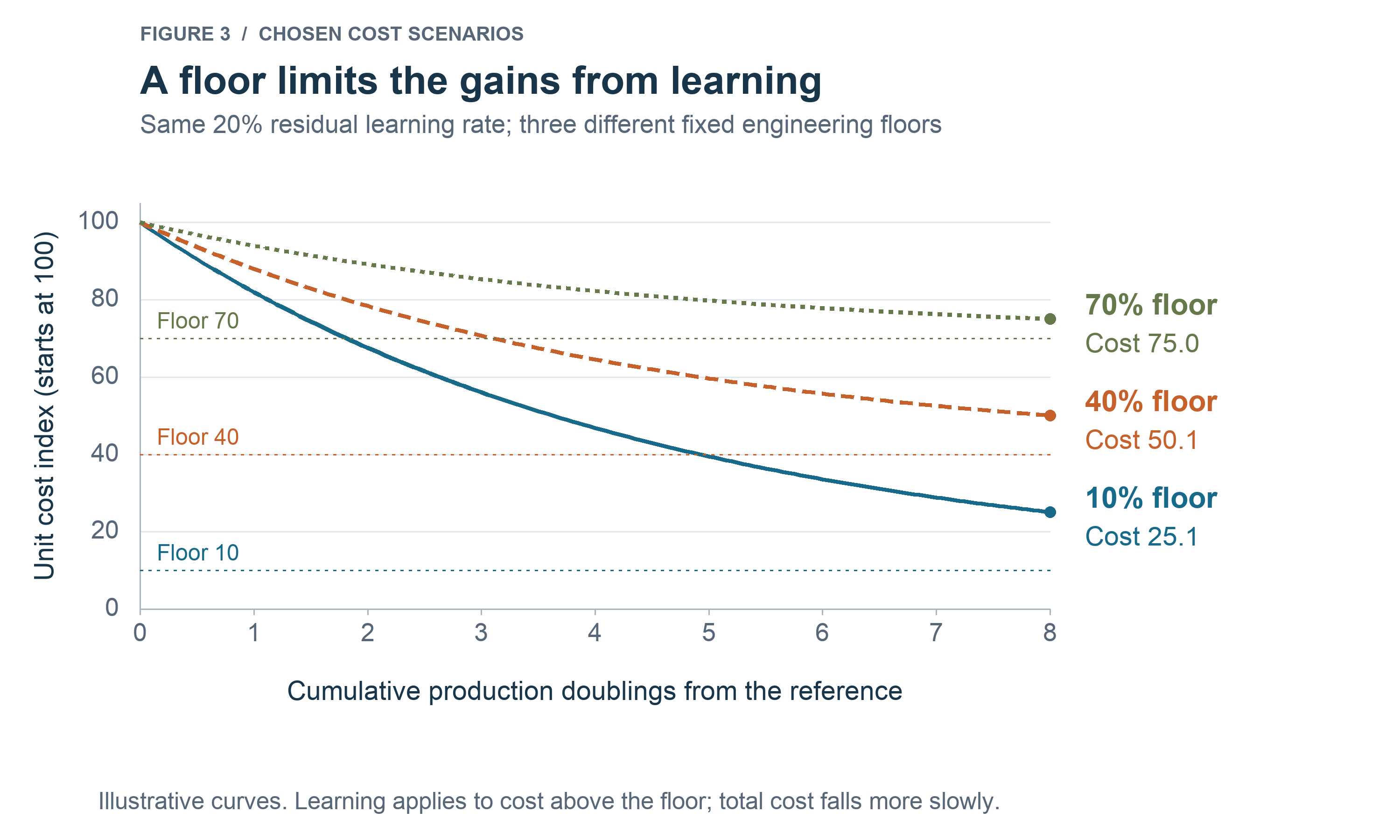
Figure 3. Three scenarios start at cost index 100 and reduce the residual by 20% per doubling, with floors of 10, 40 and 70. Figure 1 reduces total LCOE until it reaches a chosen NOAK floor. Figure 3 reduces only cost above the engineering floor. A 20% residual rate is not a 20% total-cost rate.
For a target cost C_target, the required doublings are:
D_required = ln[(C_target-F)/(C_0-F)] / ln(1-r_res)
This applies when F < C_target < C_0 and 0 < r_res < 1. The model approaches F asymptotically. If the target is close to F, changing the design or process may achieve more than producing many more copies.
The production baseline determines what those doublings require:
D = log_2(Q/Q_0)
Q_0 is reference cumulative production and Q is later cumulative production, in the same units. Moving from 100 to 800 units provides three doublings, just as moving from one to eight does. Neither says how many years that production will take.
Historical learning rates provide context, not fusion coefficients. Inflation-adjusted PV module prices fell by 26.6% per doubling of cumulative production from 1980 to 2025; lithium-ion cell prices fell by 18.9% from 1992 to 2016. Their production units were peak watts and MWh respectively (Fraunhofer ISE, 2026a; Ziegler and Trancik, 2021). These total-price rates combine production experience, research, investment and market changes. They cannot simply be applied to a fusion component’s residual cost. Experience curves can support conditional forecasts, but building more does not guarantee falling costs, as US nuclear construction demonstrates (Nagy et al., 2013; Lafond et al., 2018; Eash-Gates et al., 2020).
REBCO: from tape savings to plant cost
A 40% tape-bill saving can become a 32% magnet saving and a 9.6% plant-capital saving. In this example, magnets account for 30% of initial plant capital and tape accounts for 80% of magnet cost. The cost shares, as much as the component improvement, determine the plant result.
REBCO improvements can reduce tape quantity, price per meter or both. Even the commonly quoted $/kA·m depends on critical current at a stated temperature, magnetic field and field orientation. More current per meter helps only if the magnet can use it within its structural, protection and operating limits. Faster deposition helps only if yield, uniformity and performance survive over the required length.
A 2024 DOE manufacturing award treats greater deposition throughput and higher critical current as distinct improvements. Its planning baseline is about $50 million of equipment for 1,000 km/year of tape capacity. That is a development-plan assumption, not a current supplier quotation, but it identifies an investment that must precede greater output (DOE, 2024).
For the calculation, assume a qualified design change reduces tape quantity by 25%, and a separate manufacturing improvement reduces price per meter by 20%. The tape bill becomes 0.75 × 0.80 = 0.60, or 60% of the original tape bill. With other magnet costs unchanged, magnet cost becomes 0.80 × 0.60 + 0.20 = 0.68 of its original value. Plant capital then becomes:
K/K_0 = 0.70 + 0.30 × 0.68 = 0.904
K_0 is original plant capital and K is revised capital, with other accounts fixed. The result is a 9.6% reduction. Figure 4 follows the same improvement through all three accounts.
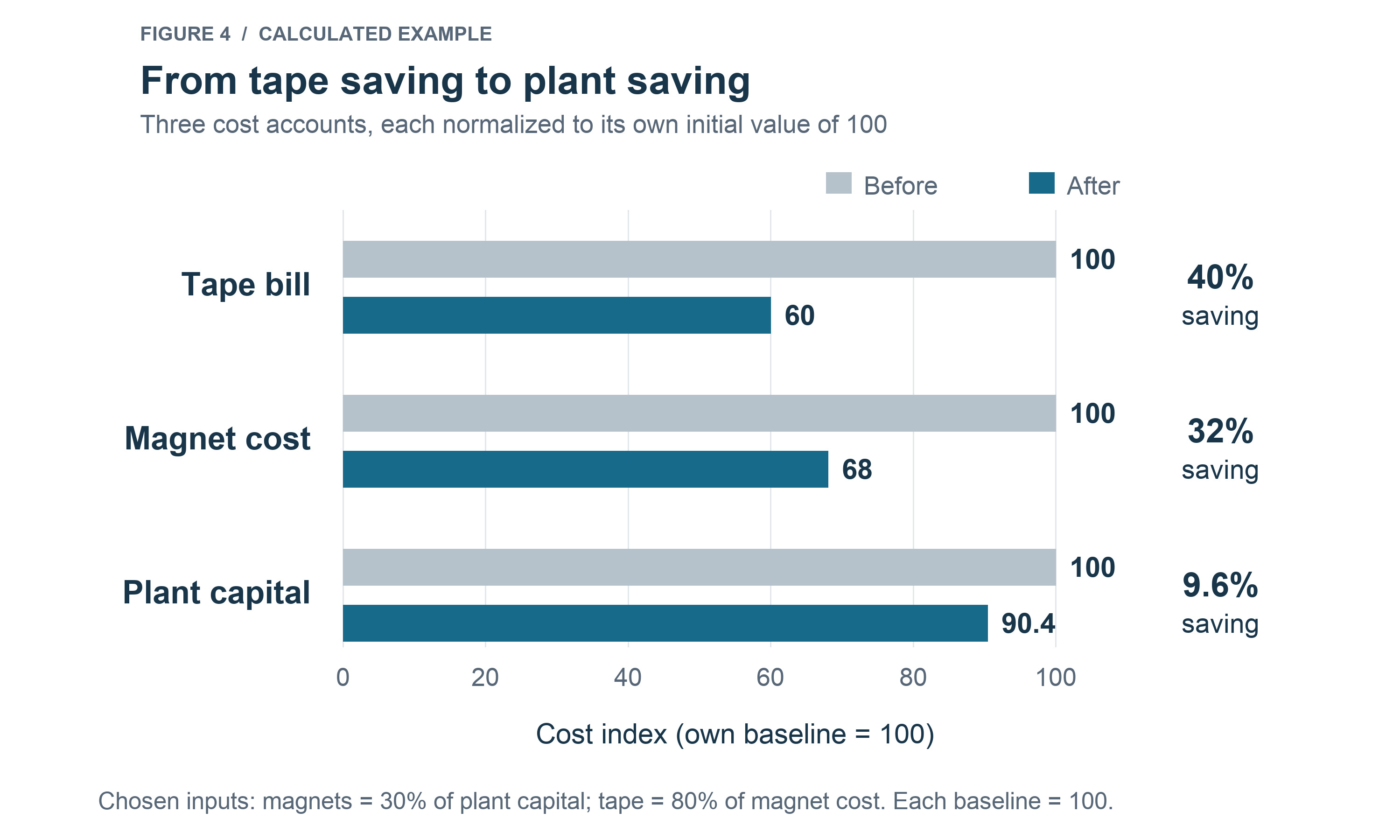
Figure 4. Calculated REBCO scenario using the stated cost shares and improvements. Each bar is normalized to its own starting cost. Other magnet and plant costs remain fixed. These are capital savings before changes in integration, operation and financing.
The price-per-meter reduction excludes the critical-current gain represented by lower tape quantity. Counting that same gain again through a lower $/kA·m would overstate the saving. A mature reference price already includes earlier learning. Further reductions need a stated additional improvement or production baseline.
After component savings are included, applying a whole-plant learning discount to those same accounts counts the improvement again. Installation and commissioning can improve separately when their costs and mechanisms are identified separately.
The supplier still needs qualified tape performance, manufacturing yield, financed capacity and enough orders to use it. The developer needs a magnet that uses the improvement at the required reliability and service life. Supplier investment must be recovered once, without counting it in both tape prices and a separate plant allowance. Capital savings become LCOE savings only after accounting for net output, replacement, downtime and financing.
Where fusion’s production experience will accumulate
The next question is which production can support the assumed learning. A plant contains equipment with different suppliers, customers and production histories. Four levels help locate the experience:
Whole-plant: construction, installation and commissioning can improve across projects, provided design continuity and a capable delivery organization preserve the lessons.
Concept-specific: specialized chambers and driver assemblies may depend on one developer’s deployment program for repeat orders.
Cross-fusion: conductors, vacuum equipment and fuel-handling capabilities may serve several approaches, where specifications and qualification requirements allow improvements to transfer.
Cross-industry: power electronics, industrial gases and conventional power equipment can use experience funded by larger existing markets. Their current prices already contain earlier learning, and another production doubling may be difficult to achieve.
These levels locate experience. They do not rank the remaining savings. Tape production, coil winding and magnet integration have different production units even within one subsystem. Two customers buying tungsten do not necessarily buy interchangeable plasma-facing components. Shared specifications and test methods determine how much work transfers.
Modularity can create repeated manufacturing operations before the first plant is complete. The FOAK cost must sum the successive units as they are made, rather than pricing every unit at the final unit’s cost. But if each plant contains the same number of modules, going from one plant to two doubles both plant count and module count. More modules do not automatically create more doublings between plants. Smaller standalone plants may reach more customers while also repeating site and staffing costs.
Operating one component many times creates operating experience. Manufacturing replacements creates new production, but also expenditure and possible downtime. A pulse count is not a count of manufactured units.
Figure 5 shows component assumptions to test. The bands are chosen screening scenarios, with a zero-learning comparison for every component. A large multiplier and a plausible improvement mechanism merit investigation, but the plant consequence also depends on the floor, cost share and qualified performance.
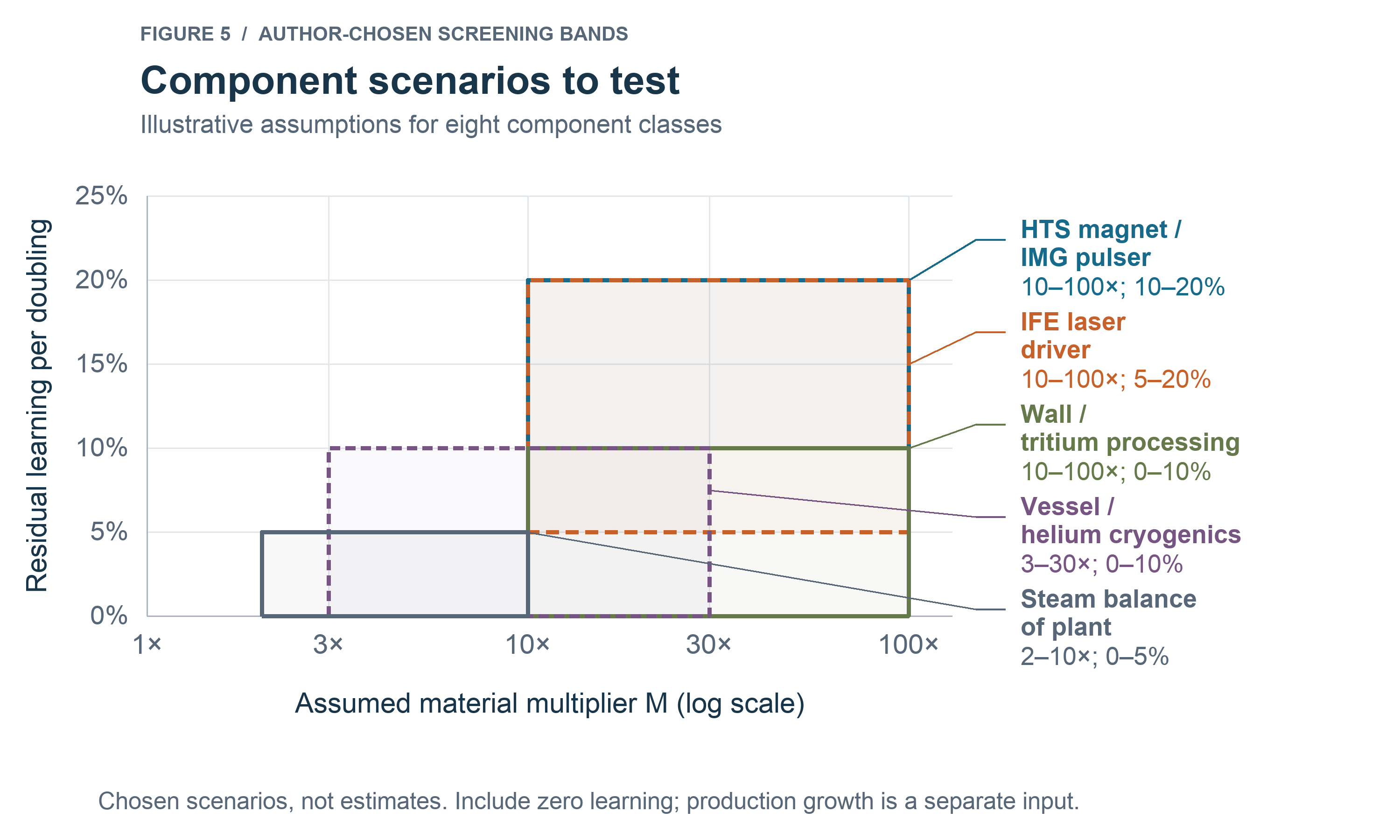
Figure 5. Material-multiplier and residual-learning bands for eight component classes. These are hypotheses, not measured coefficients or supplier estimates. Overlapping regions do not establish a ranking. HTS means high-temperature superconducting, IMG means impedance-matched Marx generator, and IFE means inertial fusion energy. The linked component matrix defines each cost boundary, including tritium processing separately from the breeding blanket and fuel inventory.
Component and whole-plant estimates need consistent cost boundaries. Tang and colleagues estimate about a 2% to 8% reduction in whole-plant specific capital cost per doubling of cumulative installed capacity for selected magnetic and laser D-T cases, using expert judgment and historical analogies. Woodruff argues for component-level manufacturing analysis. A whole-plant rate cannot be reassigned to installation alone while component savings are applied elsewhere. Nor do those selected cases establish a rate for every fusion architecture (Tang et al., 2026; Woodruff, 2026).
The component matrix retains all eight sets of assumptions. Our plant-economics work and 1costingFE introduction describe how component and integration assumptions enter a common cost model.
What fusion can learn from PV and concentrating solar
PV had customers for expensive early output and a small manufacturing unit that could serve progressively larger markets. Space applications valued reliable power. Remote uses valued avoiding fuel delivery or grid connections. Subsidized residential installations and then larger grid markets expanded demand. Germany’s feed-in tariffs provided revenue certainty at prices that ordinary wholesale electricity sales would not have supported (DOE, n.d.; IEA PVPS, n.d.; Fraunhofer ISE, 2026b).
A rooftop installation and a utility-scale plant could buy modules from the same factories. Growing demand supported manufacturing investment and allowed improvements to transfer across applications. Research, higher efficiency, lower material use and larger factories also contributed to falling module costs (Kavlak et al., 2018).
Concentrating solar power, CSP, also improved. IRENA’s global series puts newly commissioned utility-scale PV at $417/MWh in 2010 and $43/MWh in 2024. CSP fell from $402/MWh to $92/MWh over the same period, all in 2024 dollars (IRENA, 2025).
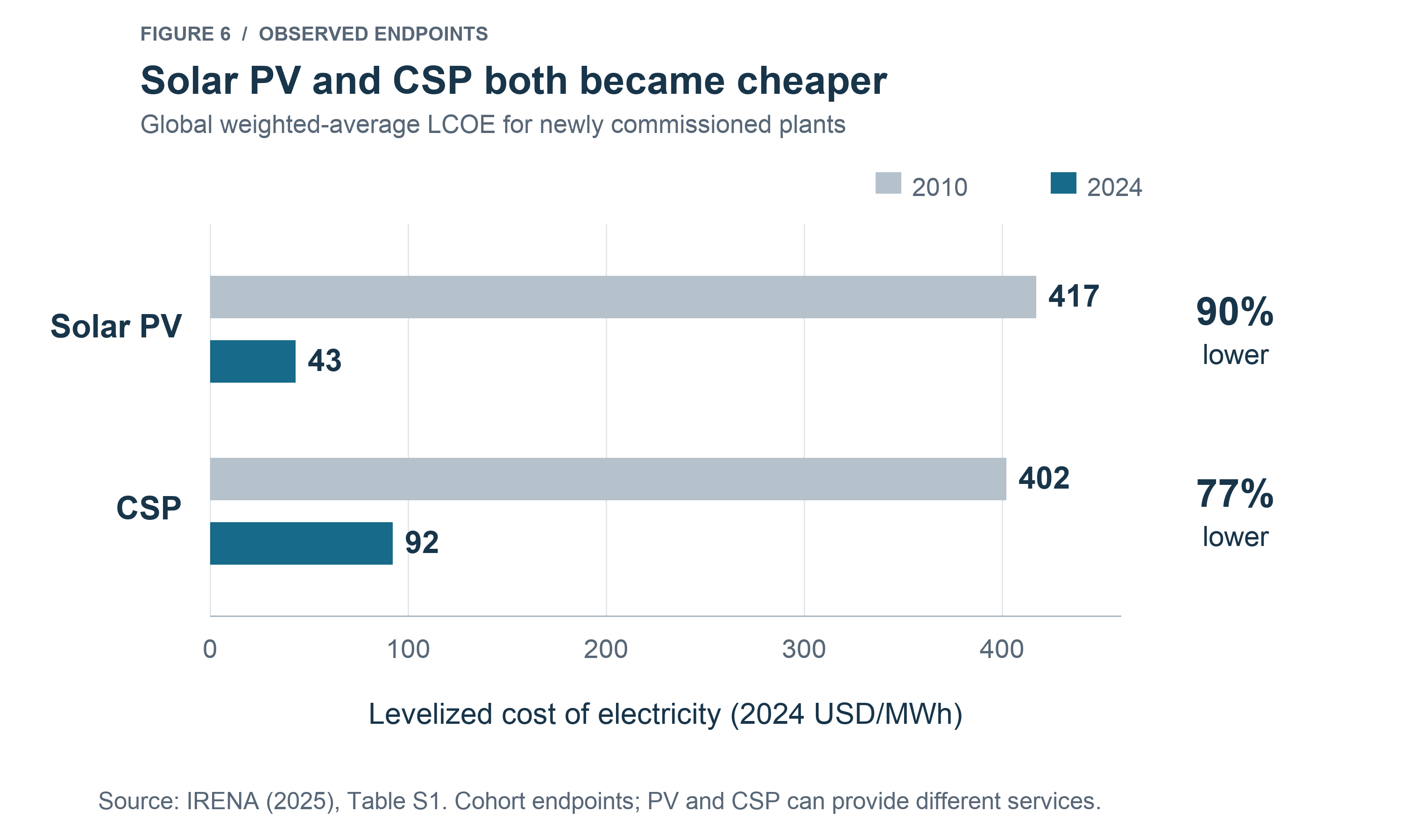
Figure 6. Observed IRENA LCOE endpoints for newly commissioned plants. CSP increasingly includes thermal storage and can supply a different generation profile. These endpoints show cost reductions in both technologies; they do not isolate the effects of modularity, policy or production experience.
CSP’s mirrors, receivers and power-cycle equipment show why industrial plants should not be treated as incapable of improvement. PV shows the advantage of a repeatable unit with customers across applications and project sizes. For fusion, the relevant questions are which qualified units can serve other markets, and how much production those markets can support before electricity sales become competitive.
Why fusion’s improvement path is hard
Fusion must improve a complicated and complex plant while finding customers for its early output. Complicated describes the number of parts and operations. Complex describes how their interactions and feedback affect the whole system. Stable interfaces can allow independent improvements to a complicated assembly. Strong coupling makes that harder: a change to one part can require changes elsewhere before system performance improves.
Plasma behavior, confinement, heating, fueling and surrounding structures interact. Better conductor performance does not automatically produce a cheaper plant. Protection, stress limits or operating conditions may have to change too. Work on design complexity explains how an improvement to one component can worsen a system through its connections to others (McNerney et al., 2011). Standardization and qualification can make more improvements transferable, but each must be checked at the plant level.
Our free-core analysis isolates the cost burden remaining even if the fusion core were free. The direct-conversion discussion considers changing the equipment the plant needs. These are questions about system requirements as well as manufacturing cost.
Investment and customers
Before a factory can learn from repeated production, someone must pay for equipment, process development and qualification. Expansion needs orders that use the resulting capacity. Dedicated equipment can reduce labor and variability, but a design change can make it unusable. Large batches can simplify qualification while delaying adoption of the next improvement.
Knowledge can also be lost when people leave, suppliers change or production stops. Aircraft-production research finds organizational forgetting and incomplete transfer between models (Benkard, 2000). Stable teams, records and compatible specifications help preserve learning. Research budgets and investor capital can support early production, but still need a route to customers at the required volume.
Electricity already has alternatives. We should expect most available firm-power substitutes to cost substantially less than FOAK fusion. Some customers may pay more for firm, low-carbon output from a compact site, or a lower long-term radioactive-waste burden than fission. Faster permitting and construction with less local opposition could also be valuable. These possibilities depend on the design and site. Fusion can still produce radioactive waste, including activated structural materials (Gonzalez de Vicente et al., 2022).
The question is how much demand those advantages create. One premium-paying customer helps only if subsequent orders support the production needed for further cost reductions.
What demand support could do
Public procurement, contracts for difference or production credits can cover a gap between early costs and customers’ willingness to pay. Figure 1 shows how starting cost and learning rate change the required amount.
The hypothetical market buys four plants’ output at up to $240/MWh, twelve more at up to $140/MWh, and further output at $80/MWh. B and C start at $220/MWh with total-LCOE learning rates of 20% and 15%. B’s 17th plant costs about $88/MWh and C’s fifth about $151/MWh. Both therefore stop before the next customer can support the next plant.
Additional support lets them continue. Summing each plant’s contracted electricity multiplied by its positive price gap gives about $447 million for B and $11.2 billion for C. Their new plants become competitive at plants 24 and 75, before reaching NOAK. These are undiscounted commitments over 20-year contracts, not annual subsidies or complete commercialization budgets. Existing contracts remain payable after new plants become competitive. Supplier investment, failed projects, deployment timing and financing require separate treatment.
Germany provides a historical comparison: cumulative PV feed-in-tariff differential costs reached about €100 billion through 2020, above electricity-sales revenue (Fraunhofer ISE, 2026b). The SCSP’s proposed one-time $10 billion fusion investment emphasizes research, infrastructure and demonstration, which address a different need from payments supporting repeated commercial output (SCSP, 2025).
Research funding can test whether an improvement works. Procurement can support production once a qualified design and credible delivery path exist. Paying for deployment too early can repeat an expensive design without delivering the intended improvement. Support needs financeable terms and evidence requirements for qualification, delivered output and unit cost, with clear decisions when milestones fail.
AI and learning rates
Better tooling and AI could lower the first plant’s cost, shorten the time between plants, or increase the cost reduction achieved per production doubling. All three could improve the commercial path, but they are different economic effects.
The learning-rate effect can be large. In the magnet example, reducing the residual by 10% per doubling requires about 20.9 doublings to reach $2 million. At 20%, it requires 9.85. The floor and target are unchanged. This calculation reduces the number of doublings by just over half, not the production volume or elapsed time by half. It illustrates the value of faster learning, not an estimate of what AI will achieve.
Engineering teams learn by observing deviations, diagnosing causes, testing changes and adopting those that work. Manufacturing research finds learning embedded in organizations and production systems as well as individuals (Levitt et al., 2013). Tools that connect test results, production records and design decisions could help retain knowledge and extract more useful improvements from each unit.
The Multi-Agent Design Assistant coordinates language-model agents and simulation tools for inertial-fusion design studies (Shachar et al., 2026). It demonstrates computational design assistance. A simulated improvement still requires manufacture, testing and qualification before it becomes a cheaper plant.
For 1cFE, the useful measurements include engineering time per accepted change, experiments needed to meet a specification, yield and qualified cost. Faster simulation alone does not establish a higher manufacturing learning rate. If better tools do increase the reduction achieved per production doubling, the same early demand could support a larger cost improvement. Lowering FOAK cost could also let a design enter markets it otherwise could not serve.
The path to 1¢/kWh
A plausible 1¢/kWh fusion NOAK would be an exciting prospect. Without an economically plausible path from the first plants, it remains a theoretical target.
Material multipliers identify manufacturing costs to investigate. Engineering floors, cost shares and production baselines determine how much improvement is available and what it would do to the plant. Customers and investment determine whether enough qualified production can occur. Figure 1 shows why a lower mature cost can coexist with a less viable route to competitiveness. The curves here are scenarios. We have not measured a commercial fusion learning rate.
Better tooling and AI may change that calculation by lowering initial costs or increasing the improvement achieved through each production doubling. That possibility deserves investigation alongside the physics and engineering of the mature plant.
The 1cFE question is whether there is a plausible 1¢/kWh NOAK and a plausible path to get there. Faster learning could make that path possible.
Calculation notes
Wright’s 1936 aircraft study helped establish the relationship between production experience and unit cost. The familiar power-law form relates cost C to cumulative production Q, relative to reference values C_0 and Q_0:
C(Q) = C_0 × (Q/Q_0)^(-b)
The exponent b determines the total-cost learning rate r:
r = 1 - 2^(-b)
If cumulative production doubles n times in a year, the corresponding annual reduction is:
Annual cost reduction = 1 - (1-r)^n
At a 20% total-cost rate, three doublings leave 51.2% of the reference cost. If they occur in one year, the annual reduction is 48.8%. A rate per doubling alone supplies no calendar schedule (Wright, 1936). These total-cost identities are distinct from the residual model used in Figure 3 and the magnet example.
Data and sources
The public GitHub repository contains the plotted data, editable figures, calculation scripts and source notes. The Figure 1 model records the demand and support assumptions. The Figure 2 inputs retain the car and house accounting boundaries. The learning-rate sensitivity records the magnet calculation at 10% and 20%. Published observations retain their units and price years; chosen scenarios retain their inputs. Questions and corrections are welcome through our contact page.
Conflict of interest
Damien Scott is a co-founder of Borealis Fusion, a company developing proton-boron-11 fusion. Astera Institute is an investor in Borealis Fusion.
References
Benkard, C. L. (2000). Learning and Forgetting: The Dynamics of Aircraft Production. American Economic Review, 90(4), 1034-1054. doi:10.1257/aer.90.4.1034.
CBO (Congressional Budget Office) (2022). Prescription Drugs: Spending, Use, and Prices. January, Box 3. Report.
DOE (U.S. Department of Energy) (2012). Report on the First Quadrennial Technology Review: Technology Assessments. Current Lightweighting Technology, p. 25. Report.
DOE (2024). High-throughput manufacturing of REBCO superconductor tapes. AMPeers LLC, SBIR Phase II award DE-SC0023996. Award abstract and development plan. Award record.
DOE (n.d.). The History of Solar. Historical timeline. Accessed 24 September 2026. Timeline.
Eash-Gates, P., Klemun, M. M., Kavlak, G., McNerney, J., Buongiorno, J., and Trancik, J. E. (2020). Sources of Cost Overrun in Nuclear Power Plant Construction Call for a New Approach to Engineering Design. Joule, 4(11), 2348-2373. doi:10.1016/j.joule.2020.10.001.
Fraunhofer ISE (2026a). Photovoltaics Report. Price experience curves, pp. 53-54. Accessed 24 September 2026. Report.
Fraunhofer ISE (2026b). Wirth, H. Recent Facts about Photovoltaics in Germany. August 2026 edition consulted, sections 4 and 5.1. Report.
Gonzalez de Vicente, S. M., et al. (2022). Overview on the management of radioactive waste from fusion facilities: ITER, demonstration machines and power plants. Nuclear Fusion, 62, 085001. doi:10.1088/1741-4326/ac62f7. UKAEA source.
IEA PVPS (n.d.). Reliability Study of Grid Connected PV Systems. Task 7 report, section 3.1 on the German 1000-Roofs Programme. Accessed 24 September 2026. Report.
IRENA (2025). Renewable Power Generation Costs in 2024. International Renewable Energy Agency. Figure 6 uses executive-summary Table S1, in 2024 USD. Report and data.
Isaacson, W. (2023). Elon Musk. Simon & Schuster. Publisher. Chapter 59, Raptor costs. Publisher-authorized excerpt.
Kavlak, G., McNerney, J., and Trancik, J. E. (2018). Evaluating the causes of cost reduction in photovoltaic modules. Energy Policy, 123, 700-710. doi:10.1016/j.enpol.2018.08.015.
Lafond, F., Bailey, A. G., Bakker, J. D., Rebois, D., Zadourian, R., McSharry, P., and Farmer, J. D. (2018). How well do experience curves predict technological progress? A method for making distributional forecasts. Technological Forecasting and Social Change, 128, 104-117. doi:10.1016/j.techfore.2017.11.001.
Levitt, S. D., List, J. A., and Syverson, C. (2013). Toward an Understanding of Learning by Doing: Evidence from an Automobile Assembly Plant. Journal of Political Economy, 121(4), 643-681. doi:10.1086/671137.
McNerney, J., Farmer, J. D., Redner, S., and Trancik, J. E. (2011). Role of design complexity in technology improvement. Proceedings of the National Academy of Sciences, 108(22), 9008-9013. doi:10.1073/pnas.1017298108.
Nagy, B., Farmer, J. D., Bui, Q. M., and Trancik, J. E. (2013). Statistical basis for predicting technological progress. PLOS ONE, 8(2), e52669. doi:10.1371/journal.pone.0052669.
Potter, B. (2025). The Origins of Efficiency. Stripe Press. Publisher.
Potter, B. (2026). Where Are the Economies of Scale in Homebuilding? Construction Physics, 28 May. US house construction-cost breakdown from Craftsman’s National Construction Estimator; footnote 4 distinguishes purchased components from raw materials. Analysis.
SCSP (2025). Fusion Forward: Powering America’s Future. Final report, 9 October 2025, section 2.2. Release. Report.
Shachar, M. H., et al. (2026). Multiagent design assistant for the simulation of inertial fusion energy. Physical Review E, 114(2), 025303. doi:10.1103/c6jc-fnkm. Author manuscript.
Tang, L., Noll, B., Panda, A., and Schmidt, T. S. (2026). Fusion power experience rates are overestimated. Nature Energy, 11, 926-934. doi:10.1038/s41560-026-02023-8.
Woodruff, S. (2026). Component-level learning curves in fusion energy cost projections. Open letter dated 4 April, addressed to the editor of Nature Energy and publicly shared by Woodruff Scientific. LinkedIn post.
Wright, T. P. (1936). Factors affecting the cost of airplanes. Journal of the Aeronautical Sciences, 3(4), 122-128. doi:10.2514/8.155.
Ziegler, M. S., and Trancik, J. E. (2021). Re-examining rates of lithium-ion battery technology improvement and cost decline. Energy & Environmental Science, 14, 1635-1651. Table 1. doi:10.1039/D0EE02681F.
Originally published at 1cf.energy.